Wind Turbine Controllers / Fast and Simulink

A tutorial on how to simulate Wind Turbine controllers using NREL's Fast and Matlab/Simulink

---

Project maintained by borgestassio Hosted on GitHub Pages — Theme by mattgraham

State Observer

We’ll learn how to implement the state space observers in this section. A more detailed mathematical model, i.e. greater number of states, allows the system to be better represented thus allowing the controller to take into consedarion more aspects of the system and provide better results. However, some states cannot be measured, either limited by the technology availability or costs.

To solve the issue and allow the system to be controllable with a grater number of states but with limited measurements, we use a state observer. Again, I won’t go in details about this method on this tutorial, but you can find information about this in any control engineering textbook.

We start with the 3 States system because we use the Drive Train Torsion and its derivative which is usually not available as a measurement in a WT (someone correct me, if I’m wrong, please).

3 States + Disturbance Accomodating Control (DAC)

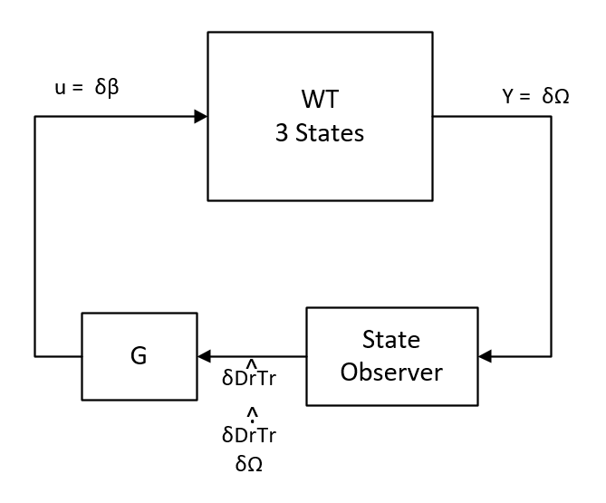
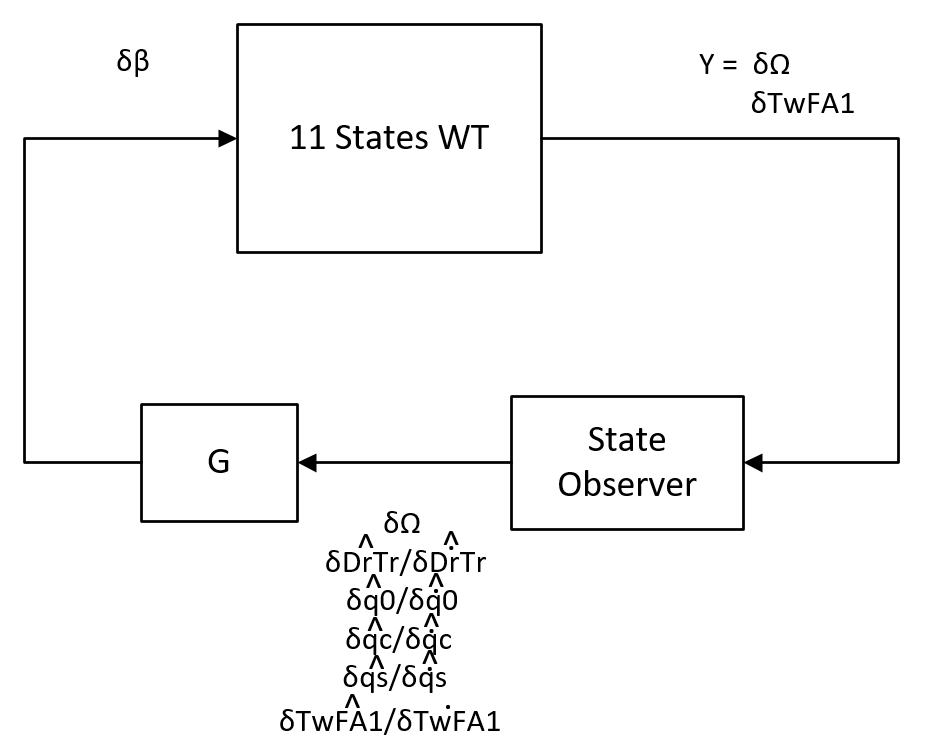
We know that some measurements are not available, whether it’s due to technological challenges or simply prohibitive costs, but a more accurate model of the system contains a number of states that cannot be measured. Therefore, to allow the use of a state feedback controller,we need to estimate the unmeasured states. On the 3 States model we’ve extracted, the only state directly available is the rotor speed, so we need to use this variable to estimate the other two (Drivetrain Torsion and its derivative). The block diagram for this controller:

There are several textbooks that explain this topic, we’ll limit to present only the expression for the state space representation with the state observer.

Where:

The observer gain Ke can be obtained either by pole placement or by LQR. In this example we’ll use pole placement, and you can find the LQR method on the states_3_observer.m file.

We also look into using the Disturbance Accommodating Control (DAC) to allow the system to react when facing a disturbance, this would take the system closer to its OP, thus allowing a better perfomance in controlling the rotor speed. I won’t go into details about this technique as we focus on implementing the controllers, but if you want to learn more, I based this controller on the one developed by Alan Wright on Modern Control Design for Flexible Wind Turbines.

The DAC approach is under the state observer section simply because it’s an augmentation of the observer, where we estimate the wind speed.

When including the disturbances, the state space representation is:

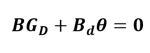
Bd is provided with the linearization as well. So we need to find Kd and Gd, which are the observer and feedback gain, respectively, to the wind disturbance. This is achieved by:

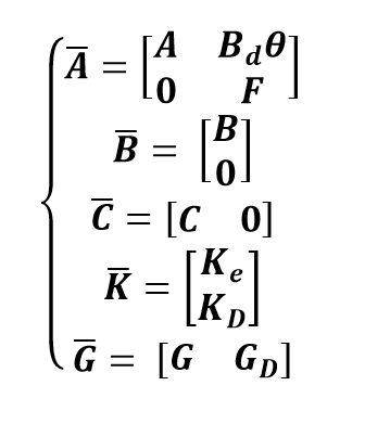
We need to find a standard space state representation that includes the disturbance, so we have:

Where Ke is the observer gain, Kd is the wind disturbance observer gain, Gd is the feedback gain for the wind disturbance observer. These values can either calculated from a pole placement or LQR.

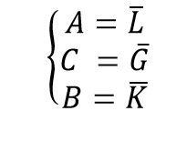
In order to allow the easier implementation of this method, we simplify the representation to a regular state space:

Where:

You can see the design of this observer and controller + DAC on states_3_estimator.m.

5 States + DAC

We already understand the 5 States model, so we assume only rotor speed is measured and we estimate the other states. I won’t go into details about this because it’s the same principle as the previous controller and the states were described in the other section.

9 States Model CPC + DAC

Note: In here, we keep using a collective pitch controller (CPC), but we’ll see Individual pitch controller (IPC) later.

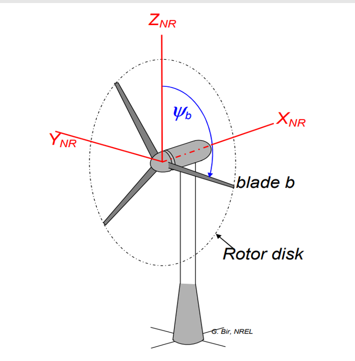
The 9 states model is fairly interesting because we use the Multi-Blade Coordinate Transformation (MBC) to change the coordinate systemfrom the a rotating frame to a non-rotating frame. This transformation is used to attenuate the problem caused by the linearization method, where the matrices are calculated several times during a single rotor rotation and their averages are used to create the state space representation of the linearized system. The main problem with this approach is that by using the average, the periodic terms that contribute to the system dynamics are eliminated. The proposed technique is that the average only be calculated after the MBC transformation. User’s Guide to MBC3 : Multi-Blade Coordinate Transformation Code for 3-Bladed Wind Turbines by Bir has a more detailed explanation and is worth reading.

The MBC transformation alters the DOFs from the rotational plan to the non-rotational plan coordinates (Xnr, Ynr and Znr) as in the figure below extracted from the aforementioned MBC3 User’s Guide:

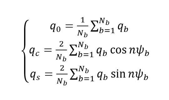
The states obtained from the MBC are:

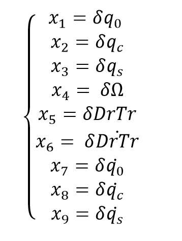
Where q0 is the rotor collective lag, qc is the horizontal displacement of the rotor center-of-mass in the rotor plane and qs is the vertical displacement of the rotor center-of-mass in the rotor plane. These are the states we’ll have for the 9 states model:

The files necessary to implement this controller are available on this repository, under the files folder, as usual.

11 States Model MBC CPC + DAC

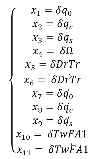
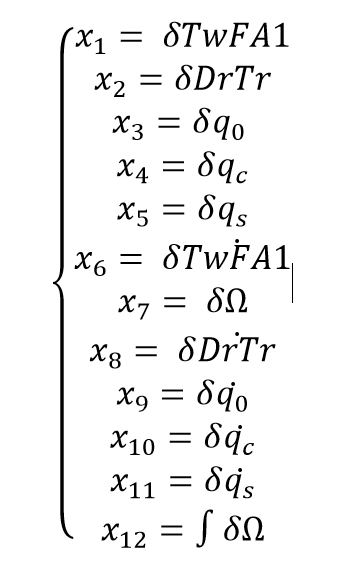
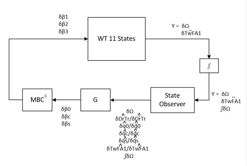
For the 11 States model, we add the 1st tower fore-aft mode DOF (TwFA1) and its derivative. In here we assume the tower fore-aft speed is measured, therefore the C matrix has 2 lines, one for the Rotor Speed and the second one for the Tower fore-aft speed. The other states are estimated using the same technique for the state observer. The states are presented below:

The Block Diagram for this system is:

I used LQR to find the gains for the estimator and the state feedback.

You might be asking yourself at this point something like ‘why is this guy just adding DOF after DOF with no purpose?’ Well, it might seem that we have no goal here, but by adding more DOFs we get increasingly closer to what the real-world system is like. But not only that, by knowing and taking into consideration the relationship between the states when designing the controllers, we can also set the controller to control these states as well and enhance the tower fore-aft oscilation for instance. There’s a quick experiment you can run, enable all the DOFs on the WT and run the 3 states controller and this one, then compare the results.

You can also find the files for the implementation of this controller under the files folder, as usual.

11 States Model MBC IPC + DAC

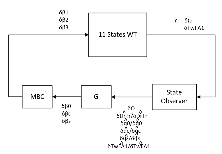
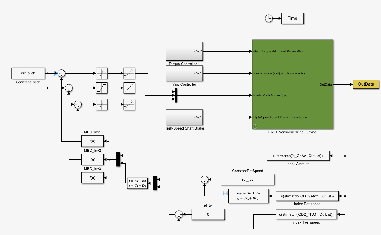
Now we’ll start to implement the Individual Pitch Control, where the controller will control the angle of each blade. The MBC transformation for the blades will transform the blades’ angle to their collective, vertical displacement and horizontal displacement components, just like what happens to the flapwise bending mode we discussed earlier. The difference here is that the controller output is actually in the Non-rotational plan, but the WT does require the angles, so we have to apply an inverve MBC transformation to get the pitch angle for each blade.

Below you can see how the block diagram looks like for this system:

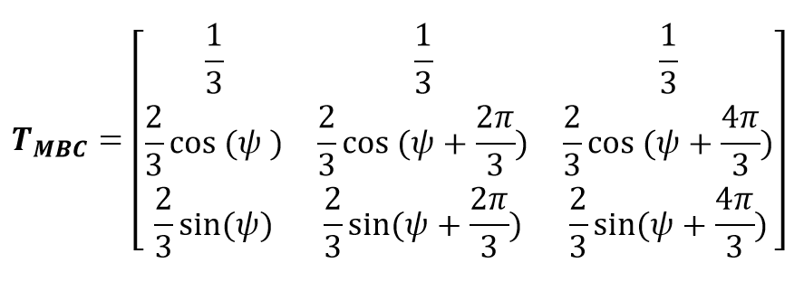
Given that we absolutely need to perform the MBC inverse transform, I present below the MBC transformation matrix:

Note that the azimuth angle (psi) is necessary, therefore it’s also needed for the inverse transformation. For the sake of brevity, we assume that the azimuth angle is measured.

In the same MBC User Guide, Bir shows how to perform the inverse transformation:

Note that the blades on this WT are 120° (2*pi/3) apart.

The states are the same as the previous model, so no changes to that.

The Simulink model is shown below:

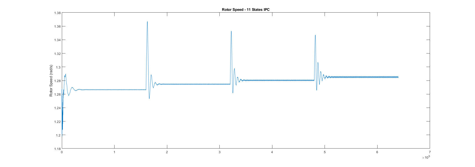
This should be the result you get for the rotor speed:

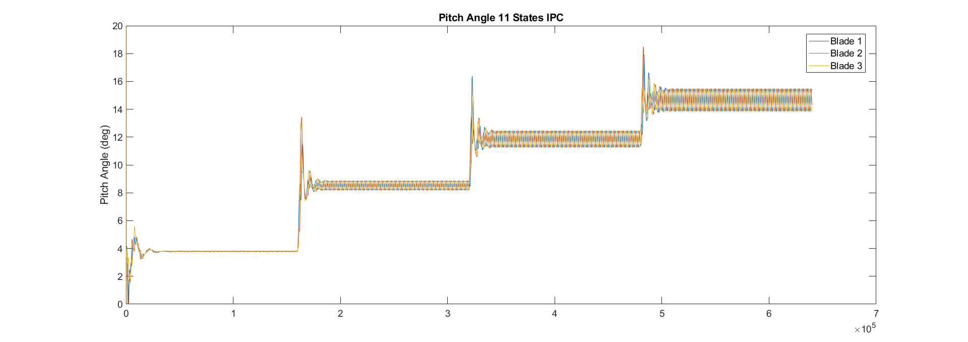
Let’s take a look at the pitch angles so we can confirm it’s actually an IPC controller:

11 States Model MBC IPC + DAC - Tower Accelaration

We assume that the tower fore-aft displacement or speed is able to be measured, however it’s more common to have an accelerometer to measure the tower fore-aft acceleration. With that in mind, we change the linearization and the matrices extraction to use the tower fore-aft accelaration instead of the speed or displacement.

We know that this variable is not among the states for the system and the linearization doesn’t provide us with this state, but there’s a workaround that allow us to get the measurement into the linearized system.

First, we need to make this measurement available on the .lin file, we do this by adding “QD2_TFA1” to the outlist on the NRELOffshrBsline5MW_Onshore_11_STATES_IPC.fst file for linearization (you can locate this file under the linerization folder for this model):

This will include the tower acceleration to the output states (y) and it’ll represent this measurement as a combination of the state space variables present on the system. If you look at the .lin file, you can locate that this measurement will be shown on the 7th line of the C matrix.

Therefore, we extract the 7th line of the MBC_AvgC matrix, so the tower acceleration is represented as a combination of all variables on the linearized system.

The Simulink model only needs to updated to measure the tower accelaration instead of speed, so we update the index to QD2_TFA1 and that’s all.

12 States (11 + Integral) Model MBC IPC + DAC

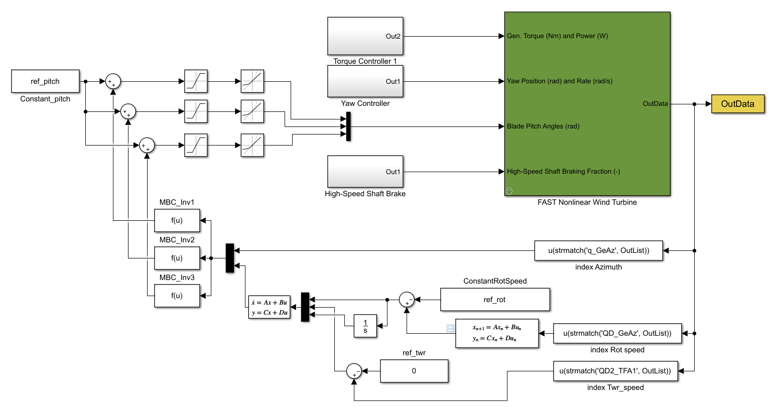
Although we’re adding more states and have a DAC to try to compensate for the wind speed, the controller is still not managing to keep the rotor speed under the desired OP. A technique we implement now is to add a integral state, with this state we can integrate the rotor error (just like the ‘I’ component of the PID) and use to correct the collective pitch component and keep the rotor speed closer to the reference value.

The state space variables for this model are:

The block diagram for this system is shown below:

The Simulink implementation:

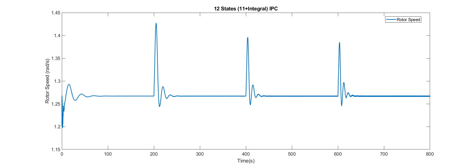
The result for the rotor speed is shown here:

See the next section to continue this tutorial and see the use of a Artificial Neural Network and Gain Scheduling.